
12 reasons why you should use Excel Tables
- Sep 11, 2017
- 9 min read
Updated: Feb 11, 2024
TABLE OF CONTENT
Why should you use Excel tables?
Reason n°2: Table headers remain visible even when you scroll down
Reason n°4: Tables automatically expand when you add new rows or columns
Reason n°7: When Tables automatically expand, they also expand...their format
Reason n°11: You can add Forms to facilitate entry of new data
Reason n°12: You can use Slicers and Timelines to filter your data and charts
About Excel tables
What is an Excel table and how to create it?
An Excel Table is not just any range of data with headings, but a specific Excel object that unlocks additional properties. Contrary to a random set of data, Tables work as a whole, something that can be very useful and make your Excel spreadsheet much easier to use, to share and to update. It usually looks like this:

How do I recognize an Excel Table?
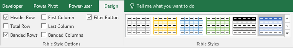
By default, Excel tables have the very distinctive appearance you can see above, with blue banded rows. However this format can be changed so it doesn't guarantee you actually have a Table. But you can know you have an Excel Table when you select a cell and the Design tab shows up on the ribbon, allowing Table-specific features, like shown in the screenshot below:

How to create a Table in Microsoft 365 Excel?
That's super easy!
Select a set of data, go to the Insert tab and click Table (or just press the "CTRL+T" keyboard shortcut). The following dialog box shows up:

Tick the checkbox "My table has headers" if there was already headers in the selected range, otherwise Excel will automatically add a headers row because Excel Tables always require to have headers.
Click OK, and the table is created. A good practice would be to go to the Design tab and rename your Table. It will be useful later when formulas or data sources refer to it.
Why should you use Excel tables?
There are many benefits to using Excel tables, because Microsoft 365 Excel recognizes that each column is a separate field. We have listed here 12 reasons why you should use Excel Tables.
Reason n°1: Tables are very easily formatted
When a Table is created, Excel automatically applies a specific formatting to it. But you can easily change this formatting:
Add or remove banded rows and columns from the Design tab, by simply ticking or un-ticking the checkboxes as shown in the screenshot below
Change the Style of the Table, using the Styles Gallery shown below
This is very easy and will let you change the Table to your preferred Style really really quick. Look on the screenshot below how the same Table can look different when simply changing the applied Style.

Reason n°2: Table headers remain visible even when you scroll down
Excel recognizes the top row of the Table as column headers. And when you scroll down, you will always see the headers, allowing you to know anytime with which column you are working, as in the screenshot below:

This is as long as your selection is within the Table, but the A,B, C letters will be displayed as usual when your selection is not within the table.
Reason n°3: Filters are added to your data
OK that's a small one, but when you create a Table, Excel will add filters to it, making it ready to use.
Reason n°4: Tables automatically expand when you add new rows or columns
If you add any data in a cell adjacent to your Table, the Table will automatically be resized to include this in a new row or column.
Important tip: Excel Tables have a little handle at the bottom-right, as you can see below:

This handle allows you to increase or decrease the size of the table manually, by simply dragging it. If you add data and the Table automatically expands, this will be useful so you can size it back to the original size. Also you can simply use the CTRL+Z keyboard shortcut after inserting data to keep the Table's original size. This will cancel just the Table's expansion and not remove the data added.
Reason n°5: Tables automatically name ranges
That's a major benefit, as we've explained in another post (Why you should name ranges in Excel and how to to it). Named ranges are really, really powerful to make Excel dynamic and user-friendly. Well the good news is, when you create a Table, Excel automatically creates names for each column, ready for you to use in your formulas.
By default, the formulas referring to ranges within a Table will be written referring to these names.
This can be a bit disturbing at first if you are not familiar with named ranges, but once you start to know how to use them it will make things much easier.
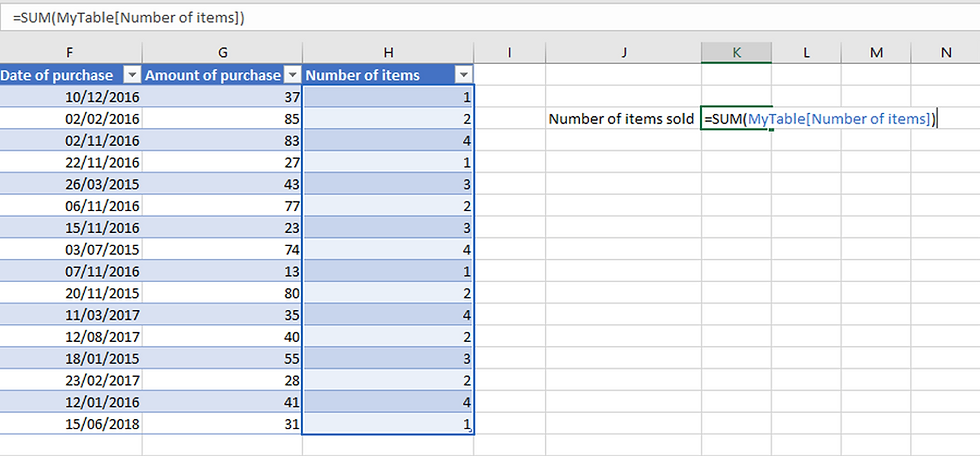
A great advantage of this is that you can share your workbook with anyone and they will quickly understand your formulas. =SUM(MyTable[Number of items]) tells you right away that you are taking the sum of all number of items, and it's much more intelligible than =SUM(Sheet1!H2:H17)
For each column, the following names are created:
MyTable[Country] can be used anywhere to designate all the data in the "Country" column of the Table called "MyTable". This does not include the header, just the data.
MyTable[@Country] looks very much the same but is really different. When there is this "@" symbol, the name means basically "in the same row". So if my formula contains MyTable[@Country] it will take for each row the corresponding country (in the same row), and not the whole list of countries every time.
MyTable[[# All];[Country]] will designate the same column as MyTable[Country], but including the header.
Now you can make it more complex and select multiple fields at once, but there is no need to know this all by heart.
Just remember that the names are created automatically, but also that they will be automatically used in the formulas referring to cells or fields within a Table.
Reason n°6: You can add Totals to Tables automatically
You can very easily add Totals to your table. Just go to the Design tab and check the "Total Row" checkbox. You can also add Totals by right-cliking your Table, then selecting "Table" and "Total Row". A row will be added at the bottom of your Table, looking like this:

You can customize the Totals row by clicking the drop-down button at the right of each cell. This allows you to summarize the data with Average, Count, Count Numbers, Max, Min, Sum, Standard Deviation, Variance and more.

Those Totals are awesome:
If you paste new data in your Table, the Totals will adjust. Also, if you paste data that exceeds the current size of the Table, the Total row will be move automatically to make room for the new data.
The Totals will only be applied to Visible cells. If you filter some of your Table's data, the Total row will only display the values based on the visible data.
You can add Totals for any column of the Table. Simply click in the Total row and use the drop-down button to define the type of Total you want.
Useful tip: when you are working within a Table, pressing Tab from the right-end cell of a column will bring you to the left cell of the next row, so that you remain within the Table. When you reach the last cell, at the bottom-right of the Table, pressing the Tab key. will add a new row to the Table. This works with PowerPoint and Word Tables as well. So when you have a Total row, use Tab from the bottom-right cell to add a new row without overwriting the Total row.
Reason n°7: When Tables automatically expand, they also expand...their format
The fact that Tables automatically adjust to new data drives the automatic adjustment of the format. The new rows or columns will take the same format as the rest of the Table, and you can again adjust it manually or using one of the suggested Styles in the Design tab. This will spare you the time to format every new column or row you add to your data.

Reason n°8: Tables drag formulas down automatically
If you type a formula in a Table column, Excel will automatically drag down the formula for the entire column. As each column is a separate field, there is indeed no reason the formulas should be different for different rows, so they will autofill down to the last row of the Table.
In the example below, we have an amount purchased by each client and the number of items in their basket. We want to computer the average price per item sold. So we simply type the division formula, and when we hit the "Enter" key, the formula is dragged down to the bottom of the Table.

Even better, as you add new rows, formulas will be automatically expanded to these new rows. This saves you the effort to drag down the formula every time new data is added. When you have a lot of rows, it's easy to forget that you need to adjust the formulas to your new data. And this can lead to errors and painful situations. So Excel Tables will also spare you this risk by automatically ensuring formulas are consistent in the entire column.
Reason n°9: You can create dynamic charts
Tables allow you to create PivotTables or PivotCharts based on your Table data. To do so, just select any cell in your Table, then go to the Insertion tab and click on PivotTable or PivotChart.

The Pivot will have the Table as Data source. The good thing is, since the Table automatically adjust to new data, so do the PivotTables and PivotCharts.
Let's illustrate this. below is our Excel Table with an associated Pivot Chart displaying the amount of purchase per year. There are currently values for years 2015, 2016 and 2017.

Now we add a new row of data with a purchase for 2018. By Simply refreshing the PivotChart (from the Analyze tab, Refresh), the chart automatically adjusts and adds a new column for 2018. Cool right?

So you can create dynamic charts that will adjust to any addition of data, a very useful tool for Excel dashboards!
Reason n°10: Tables adjust named ranges automatically
Every time you update your Table with new or additional data, the names will adjust so that any formula, PivotTable or PivotChart referring to the column will remain up to date. For instance, the name MyTable[Country] will automatically adjust to take into account any new row added to your Table. This is very helpful if you have used this name in formulas.
Reason n°11: You can add Forms to facilitate entry of new data
That's a little know trick, but if you want other users to type new entries in your Table, you may definitely want to use Excel Forms.
Forms look like this:

This will make it more user-friendly to add new data, and make it understandable even to Excel haters. You can build administrative spreadsheets where people will be typing in Forms, filling up your Excel Table without even knowing it.
There is only one problem: Forms are not available by default in Excel. So how to you get these?
You need to add the Form button to the ribbon.
To do so, follow the steps below:
Go to File/Options and then Customize the ribbon
Select "All commands" in the top left drop-down list
Select "All tabs" in the top right drop-down list
Under the Tables tab, create a "New group" from the button at the bottom right of the window. This is the location where the Form button will be added
In the left list, look for "Form"
Click "Add" and then validate with ok

You should now see the Form button in the location you defined:

Reason n°12: You can use Slicers and Timelines to filter your data and charts
Ok so pay attention now, this is a cool stuff for dashboard builders. Since Excel Tables allow you to create PivotChart, you can also add Slicers and Timelines to it.
What is that? Very useful tools to filter on your data in a very user-friendly way. That's just ideal to share your spreadsheet with other people.
To insert a Slicer or a Timeline, select your chart and go to the Analyze tab. Click either Slicer or Timeline and select the field(s) on which you would like to let the user of your workbook filter. For instance here, we want to let users visualize the amounts for any country and for any quarter. So we add a Slicer (for countries) and a Timeline (for the date of purchase). The results looks like this:

Now by simply clicking on any quarter in the Timeline, or on any country on the Slicer, the chart will automatically update to display only the desired data. And remember, it will also adjust automatically when you add new data to your Table!
Conclusion: In case this wasn't clear, you definitely should use Excel Tables every time you can!
💡For many of these reasons, Tables are an essential part of our proven methodology to build dynamic Excel dashboards.
Want to become a master of Microsoft Office 365? Try our Power-user add-in, bringing dozens of powerful features to PowerPoint and Excel to save you a tremendous amount of time!


