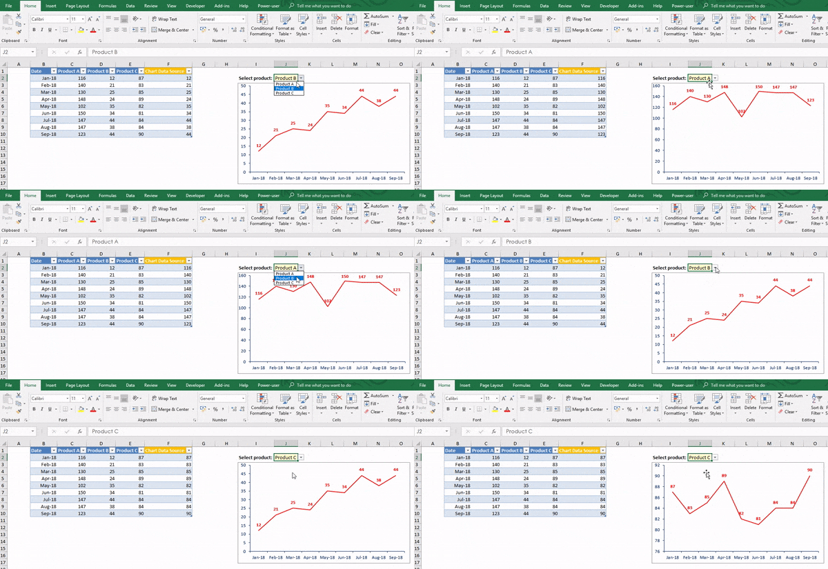
It always makes quite an impression to link a chart to a drop-down list in an Excel spreadsheet.
Imagine you are building a dashboard for reporting on your company's products sales performance. Wouldn't be great to just pick a product in a drop-down list and see the data for this product only being displayed on a chart?
But there is more to it than just showing off with a fancy workbook. Such a "drop-down chart" also enables you to use a single chart to display data from multiple series of data. This makes your spreadsheet lighter and also more efficient for the users. You can, for instance, send it to your Product Managers and each of them will be able to see the reporting for their respective product without having to search for one chart among many.

So how can you create such a chart linked to a drop-down list?
The basic idea to create such dynamic chart is actually not to link the drop-down list to the chart itself, but to its data source.
So let's get started. It's actually pretty easy.
1) First start with a set of data
In this example the data is organized in columns so that we can create an Excel Table (see the benefits of using Excel Tables). But it could as well be organized in rows. Each column here contains the data for a different product.

2) Add a new column to your data set
Let's call it "Chart Data source" here to make things crystal clear.

3) Choose a cell and create the drop-down list
In our example, we take cell "J2" and create a drop-down list using the columns titles (i.e. product names) as source. If you are unfamiliar with it, see How to create a drop-down list in Excel.
4) In the new column, type the following formula
=OFFSET([@Date];;MATCH($J$2;Table2[[# Headers];[Product A]:[Product C]];0))
or if you are not a fan of Tables, you will type instead:
=OFFSET(B2;;MATCH($J$2;$C$1:$E$1;0))

5) Now just create a chart that takes the new column as data source

That's it. Now you can play with your drop-down list in J2 and see how the chart updates.
If you are an heavy user of Microsoft Office 365, you will most certainly like the Power-user add-in. Get dozens of new advanced features that will make you the boss of Excel and PowerPoint!

